Ferri/Ferrocyanide Reaction with diffusion in Julia – Part 2

by Steven Anker · January 3, 2023

In the post Simulating Ferri/Ferrocyanide Reaction in Julia, I described my first attempt to simulate a ferry/ferrocyanide reaction in Julia by solving a so-called split-ODE, where one ODE was generated from a PDE containing the diffusion equation. The other ODE was generated from a reaction network, describing the reaction at the electrode.

One problem is that the PDE is constructed using DiffEqOperators.jl, which is deprecated. The library is replaced by MethodOfLines.jl. My old code also did not run well in a Pluto notebook. This post describes my first attempt to simulate the reaction using MethodOfLines.jl. I based my code on the example on solving the heat equation.

The following packages are used:

using OrdinaryDiffEq
using ModelingToolkit
using MethodOfLines
using DomainSets
using Gadfly

Most of the constants used in the original post are used again:

const width = 0.01
const Δx = 0.0002 # The distance between points in the cell
const Nₓ = floor(Int, width/Δx) # The amount of discrete points in the cell
const A = 1e-6
	
const F = 96485.3329 # Faraday constant
const R = 8.31446261815324 # Universal gas constant
	
const E₀ = 0.37 # standard electrode potential
const k₀ = 2.5e-4 # reaction rate constant
const T = 298.15 # Temperture
const α = 0.5
const λₐ = (-α*F)/(T*R)
const λᵦ = ((1-α)*F)/(T*R)
	
const Dₒ = 0.6e-9 # Diffusion coefficient for ferrocyanide
const Dᵣ = 0.7e-9 # Diffusion coefficient for ferricyanide

const cₘₐₓ = 1.0 # The highest initial concentration

Next I’ve created a single function, which defines the PDE, discretises it into an ODE and solves it:

function solve_reaction_diffusion(t_max, E; savelog=false, c0ₒ=0.0, c0ᵣ=cₘₐₓ)
	
    @parameters x t
    @variables cₒ(..) cᵣ(..)
	
    Dt = Differential(t)
    Dx = Differential(x)
    Dxx = Differential(x)^2

    kb(E) = k₀ * exp(λₐ * (E - E₀))
    kf(E) = k₀ * exp(λᵦ * (E - E₀))

    r(x, cₒ, cᵣ, E) = (x <= Δx) * (kf(E) * cᵣ - kb(E) * cₒ)
	
    eqs  = [
        Dt(cₒ(x, t)) ~ Dₒ * Dxx(cₒ(x, t)) + r(x, cₒ(x, t), cᵣ(x, t), E(t)),
        Dt(cᵣ(x, t)) ~ Dᵣ * Dxx(cᵣ(x, t)) - r(x, cₒ(x, t), cᵣ(x, t), E(t)),
    ]

    bcs = [
        cₒ(x, 0) ~ c0ₒ,
        cᵣ(x, 0) ~ c0ᵣ,
        Dx(cₒ(0, t)) ~ 0,
        Dx(cᵣ(0, t)) ~ 0,
        Dx(cₒ(width, t)) ~ 0,
        Dx(cᵣ(width, t)) ~ 0
    ]

    domains = [
        t ∈ Interval(0.0, t_max),
        x ∈ Interval(0.0, width)
    ]

    @named pdesys = PDESystem(eqs, bcs, domains,[x, t],[cₒ(x, t), cᵣ(x, t)])

    discretization = MOLFiniteDifference([x => Δx], t)
    prob = discretize(pdesys,discretization)

    s = savelog ? [10^i for i ∈ 0:0.2:log10(t_max)] : (0:(t_max/1000):t_max)
	
    sol = solve(prob
                , BS3()
                , saveat=s
                , save_start=true
                , abstol=1e-10
                , reltol=1e-10
                , maxiters=1e7
        )
    sol, x, t, cₒ(x,t), cᵣ(x,t)
	
end

This function has a few oddities. My initial idea, was to incorporate the reaction part of the equation in the boundary conditions like this:

eqs  = [
    Dt(cₒ(x, t)) ~ Dₒ * Dxx(cₒ(x, t)),
    Dt(cᵣ(x, t)) ~ Dᵣ * Dxx(cᵣ(x, t)),
]

bcs = [
    cₒ(x, 0) ~ c0ₒ,
    cᵣ(x, 0) ~ c0ᵣ,
    Dt(cₒ(0, t)) ~ kf(E(t)) * cᵣ(x, t) - kb(E(t)) * cₒ(x, t),
    Dt(cᵣ(0, t)) ~ kf(E(t)) * cₒ(x, t) - kb(E(t)) * cᵣ(x, t),
    Dx(cₒ(width, t)) ~ 0,
    Dx(cᵣ(width, t)) ~ 0
]

But for some reason, this does not work. All the concentrations stay at their initial value. No clue why this exactly happens. But the trick is to move the reaction part one step away from the boundary and then it works.

The output of the solver is slightly different than the first post. In order to retrieve the data I need the symbols. This is why I return those as well. Since the output is different, all the helper functions need to be updated as well:

function current(Mₒ, Mᵣ, t, E)
	
    function redox_rate(cₒ, cᵣ, E)
        η = E - E₀
        kₐ = k₀ * exp(λₐ * η)
        kᵦ = k₀ * exp(λᵦ * η)
        kₐ * cₒ - kᵦ * cᵣ
    end
	
    mₒ = @view Mₒ[2, :]
    mᵣ = @view Mᵣ[2, :]
		
    r = redox_rate.(mₒ, mᵣ, E.(t))
    b = F * A
    b .* r
end

function plot_I_vs_E(I, E)
    plot(x=E, y=I
	, Guide.xlabel("E (V)")
	, Guide.ylabel("I (A)")
	, Guide.title("I vs E")
	, Geom.line(preserve_order=true)
	, Theme(default_color="purple")
    )
end

function cv(t)
    s = 0.01
    t₁ = inv(s)
    i = floor((t - t₁)/(2t₁))
	
    (t < t₁) * (s * t + E₀) +
    (t >= t₁) * (
	(i % 2 == 0) * (-s * (t - (2i+1)*t₁) + E₀ + 1.0) +
	(i % 2 != 0) * (s * (t - (2i+1)*t₁) + E₀ - 1.0)
    )
end

I’ve rewritten the function which generates the cyclic voltammetry signal, such that it does not use an if-then-else statement anymore. Note sure if this makes a performance difference. But at least it can directly be used in the PDE this way.

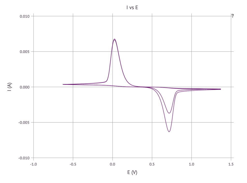
Solving the equations results in the same plot as before:

sol, x, t, cₒ, cᵣ = solve_reaction_diffusion(800, cv, savelog=false, c0ₒ=0.5, c0ᵣ=0.5)

I = current(sol.u[cₒ], sol.u[cᵣ], sol.t, cv)
E = cv.(sol.t)
plot_I_vs_E(I, E)